
(Almost) linear scaling of a star-schema query with Distributed DataFusion
A star schema with a small dimension and a large fact table is one of the most common shapes in analytics. The interesting question is not whether a query engine can join them. It is whether the plan stays streaming as the fact table grows, and whether spreading that fact table across workers buys almost-linear speedup — 10 workers close to 10× faster, 50 workers close to 50× — instead of a plan that works on many nodes but does not get faster.
This post walks through that example the way I presented it: two tables, one join, one aggregation, then the same physical plan on one node and on many.
Two tables: dimension and fact
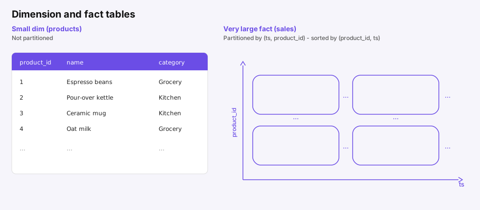
The schema is a classic many-to-one relationship. products is the dimension. sales is the fact.
products is small and not partitioned. Each row is one product. The primary key is product_id.
| product_id | name | category |
|---|---|---|
| 1 | Espresso beans | Grocery |
| 2 | Pour-over kettle | Kitchen |
| 3 | Ceramic mug | Kitchen |
| 4 | Oat milk | Grocery |
sales is large. Each row is one sale of one product at one timestamp. product_id is a foreign key back to products.
| product_id | ts | amount |
|---|---|---|
| 1 | 2026-09-01 16:10:00 | 10 |
| 1 | 2026-09-01 16:10:05 | 11 |
| 1 | 2026-09-01 16:10:10 | 8 |
| 2 | 2026-09-01 16:10:00 | 20 |
| 2 | 2026-09-01 16:10:20 | 10 |
| 3 | 2026-09-01 16:13:10 | 45 |
Two physical properties on sales matter more than the column list:
- Partitioned by
(ts, product_id). Adjacent time ranges — and the product keys that appear in them — live in different files. A time predicate can skip whole partitions. - Sorted by
(product_id, ts). Inside a partition, all sales for product 1 arrive before product 2, and each product’s rows are already in time order.
That sort order is the opposite of the partition key. Partitioning on time is what makes a historical range cheap to open. Sorting on product then time is what makes the aggregation stream.
The query: sales every 30 minutes for grocery products
The question is ordinary: for products in the grocery category, what were sales in every 30-minute window?
SELECT
  date_bin(INTERVAL '30 minutes', s.ts) AS bin,
  p.name,
  SUM(s.amount) AS sales
FROM products AS p
JOIN sales AS s
  ON p.product_id = s.product_id
WHERE p.category = 'Grocery'
GROUP BY bin, p.name;
date_bin folds each timestamp into a 30-minute bucket. category = 'Grocery' is the dimension filter — in the sample, that keeps espresso beans and oat milk. The join attaches the product name. The aggregate is a sum per (bin, name).
Because product_id is on both sides, the engine can push the first aggregation down onto sales alone, then join, then finish the grouping on the dimension column:
SELECT
  s.bin,
  p.name,
  SUM(s.amount) AS sales
FROM products AS p
JOIN (
  SELECT
    date_bin(INTERVAL '30 minutes', ts) AS bin,
    product_id,
    SUM(amount) AS amount
  FROM sales
  GROUP BY bin, product_id
) AS s
  ON p.product_id = s.product_id
WHERE p.category = 'Grocery'
GROUP BY s.bin, p.name;
The inner GROUP BY is the important rewrite. It collapses many sale rows into one partial sum per product and bin before the join. The join then sees a much smaller stream, and the outer aggregate only has to combine those partials by product name.
The single-node plan
After that rewrite, the physical plan looks like this:
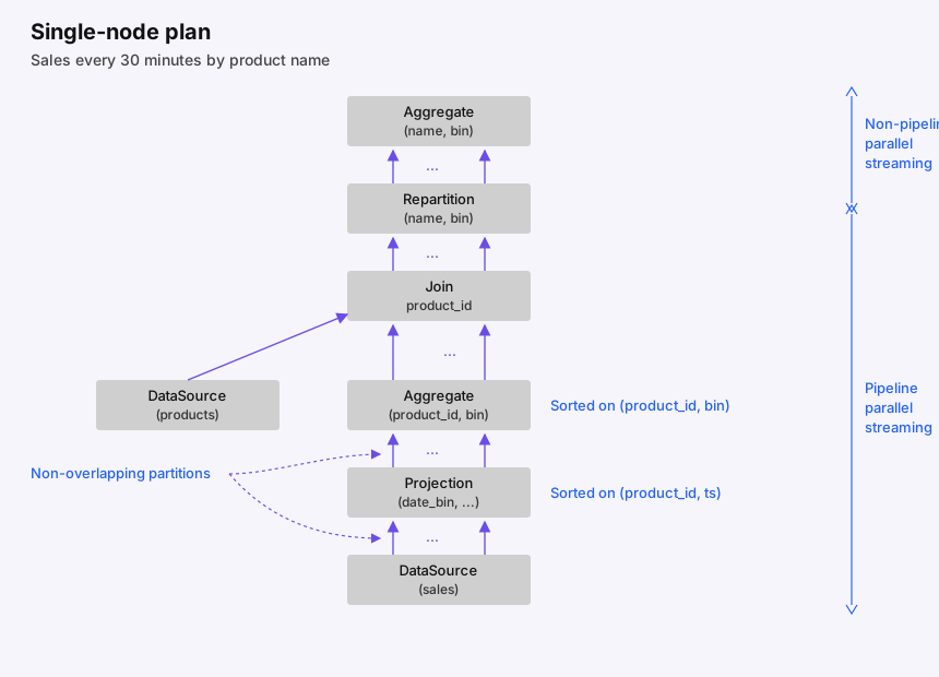
Read it from the bottom.
The sales scan opens only the time partitions that can contain the window you asked for. Those files are already sorted on (product_id, ts). After date_bin, the stream is still sorted on (product_id, bin): binning time does not reorder rows within a product. The first aggregate can therefore run in sorted mode. It does not need to hash the whole input. It emits a partial sum as soon as a (product_id, bin) group ends.
products is the small side, so it is the build side of the join: the category filter turns it into a handful of rows that fit in a hash table. sales is the large probe side, so each product_id is a straightforward lookup.
Only after the join does the grouping key change from product_id to name. That is why a hash repartition on (name, bin) sits above the join, and why the final aggregate is a second grouping, not a continuation of the first.
The partitions of sales do not overlap. Each file can run its scan, date_bin, and partial aggregate independently. DataFusion is good at this: the bottom of the plan is pipeline-parallel and streaming. Memory stays bounded, and rows leave the first aggregate as soon as they are ready.
The step above the join is different. The hash repartition has to wait for its inputs before it can send a (name, bin) group to the right partition. That upper half is not fully pipeline-streaming. For this query it is still cheap: the pushdown has already reduced the stream, and the final cardinality is one row per product per 30-minute bin.
Distributed Plan
Distributed execution does not invent a new plan. It cuts this one at the exchange.
The dimension table stays small, so each worker can read products locally. The fact table is where the bytes are. Because its partitions do not overlap, you can hand different file groups to different workers. Worker 1 reads one set of (ts, product_id) partitions; worker 2 reads another. Each worker runs the same streaming prefix: scan, date_bin, sorted aggregate, join.
The hash repartition becomes a network shuffle. Partial sums for the same (name, bin) meet on the worker that owns that hash bucket, and the final aggregate finishes there.
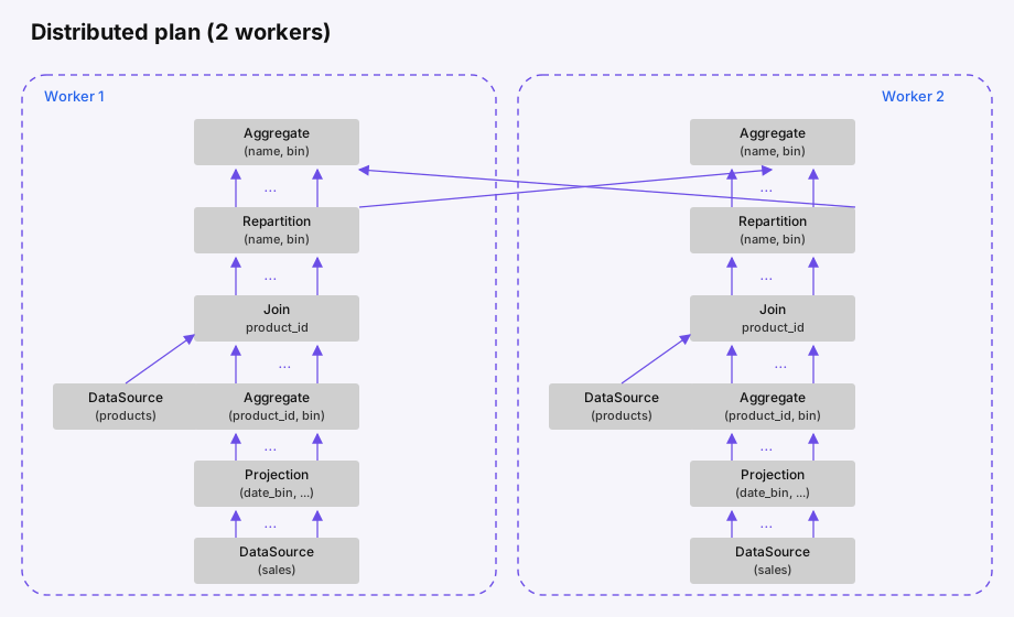
If the fact table grows, you add partitions and workers. The streaming prefix scales with the number of non-overlapping file groups. The shuffle stays small because it carries partial aggregates, not raw sales.
That is the whole trick. Partition on time so a range query opens the right files. Sort on the join key so the first aggregate streams. Push the aggregate below the join so the shuffle is tiny. Then the distributed plan is the single-node plan with an exchange drawn on the repartition.
What the numbers look like
I ran this shape of query over historical ranges from a couple of days up to 60 days, reading directly from object storage, without a disk cache in front of the scan. A single node already behaves well: the sorted partial aggregate keeps memory down, and the non-overlapping file groups keep the cores busy. The longest range was on the order of two terabytes.
The useful metric is speedup: single-node time divided by the time with N workers. Ideal linear scaling is a diagonal — 10 workers would be 10× faster, 50 workers 50× faster.
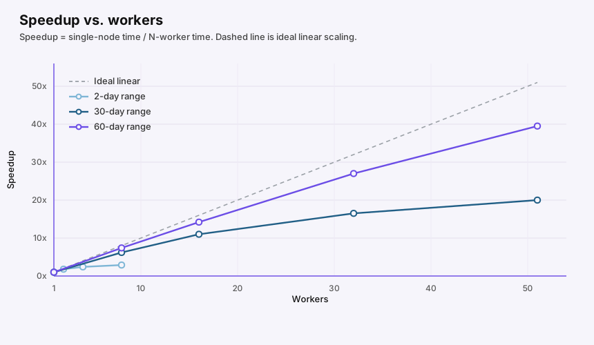
Short ranges saturate early. A 2-day window does not have enough disjoint sales partitions to keep dozens of workers busy, so speedup levels off after a handful of nodes. Stretch the same query to 30 or 60 days and the curve stays near the diagonal. At 51 workers the 60-day run is about 40× faster than one node. That is the result you want from this plan: the extra workers do more of the same streaming work on disjoint partitions, not coordinate a bigger hash table.
The cases that used to be awkward are the long, high-cardinality ones: many days, many products, many 30-minute bins. Partitioned execution is what makes those queries ordinary. Each worker only sees its slice of sales. The shuffle only sees one partial per product per bin.
What actually scales
The join is useful, but it is not what makes the plan scale. Partition sales so a range query opens disjoint files. Sort those files so the first aggregate can stream. Push work below the exchange so workers shuffle partials, not raw rows. Do that, and adding workers stays close to linear.
The same recipe applies to a single large table with no dimension at all. Drop products and the join, keep sales partitioned and sorted the same way, and a date_bin plus GROUP BY still pipelines on one node and still splits across workers. The small table is a filter and a name. The fact table’s layout is the scaling story.
Where this came from
I gave this talk at the Boston Apache DataFusion Meetup on 3 September 2026. The slides and recording cover the same example. The meetup notes and discussion live in apache/datafusion#21541.
Distributed DataFusion is the library that adds the network operators — shuffle, coalesce, broadcast — on top of Apache DataFusion. For a deeper look at how those operators are built, see the New York meetup talk by Gene Bordegaray and Jayant Shrivastava.
Comments